RL Theory 📌
Effective analysis is very hard in RL without strong assumptions
Trick is to make assumptions that admit interesting conclusions without divorcing us (too much) from reality
What is the point:
Prove that our RL algorithms will work perfectly every timeUsually not possible with current deep RL methods, which are often not even guarenteed to converge Understand how errors are affected by problem parametersDo larger discounts work better than smaller ones? If we want half the eror, do we need 2x the samples, 4x, or something else? Usually we use precise theory to get imprecise qualitative conclusions about how various factors influence the performance of RL algorithms under strong assumptions , and try to make the assumptions reasonable enough that these conclusions are likely to apply to real problems (but they are not guarenteed to apply to real problems)
⚠️
Don’t take someone seriously if they say their RL algorithm has “provable guarantees”
the assumptions are always unrealistic
Exploration Performance of RL is greatly complicated by exploration - how likely are we to find potentially sparse rewards?
Theoretical guarantees typically address worst case performance ⇒ but worst case exploration is extremely hard 🧙🏽♂️
Goal: Show that exploration method is
P o l y ( ∣ S ∣ , ∣ A ∣ , 1 / ( 1 − γ ) ) Poly(|S|, |A|, 1/(1-\gamma)) P o l y ( ∣ S ∣ , ∣ A ∣ , 1/ ( 1 − γ )) If we “abstract away” exploration, how many samples do we need to effectively learn a model or value function that results in good performance?“generative model” assumption: assume we can sample from P ( s ’ ∣ s , a ) P(s’|s,a) P ( s ’∣ s , a ) ( s , a ) (s,a) ( s , a ) “oracle exploration” assumption: For every ( s , a ) (s,a) ( s , a ) s ’ ∼ P ( s ’ ∣ s , a ) s’ \sim P(s’|s,a) s ’ ∼ P ( s ’∣ s , a )
Basic Sample Complexity Analysis RL Theory Textbook. Agarwal, Jiang, Kakade, Sun. https://rltheorybook.github.io
“Oracle Exploration”: for every ( s , a ) (s,a) ( s , a ) s ’ ∼ P ( s ’ ∣ s , a ) s’ \sim P(s’|s,a) s ’ ∼ P ( s ’∣ s , a )
Simple “model-based” algorithm
P ^ ( s ’ ∣ s , a ) = # ( s , a , s ’ ) N \hat{P}(s’|s,a) = \frac{\#(s,a,s’)}{N} P ^ ( s ’∣ s , a ) = N # ( s , a , s ’ ) Count number of transitions Given π \pi π P ^ \hat{P} P ^ Q ^ π \hat{Q}^\pi Q ^ π We want to measure worst case performanceHow close is Q ^ π \hat{Q}^\pi Q ^ π Q π Q^\pi Q π How close is Q ^ ∗ \hat{Q}^* Q ^ ∗ P ^ \hat{P} P ^ Q ∗ Q^* Q ∗ P P P How good is the resulting policy?
“How close is Q ^ π \hat{Q}^\pi Q ^ π Q π Q^\pi Q π
∣ ∣ Q π ( s , a ) − Q ^ π ( s , a ) ∣ ∣ ∞ ≤ ϵ max s , a ∣ Q π ( s , a ) − Q ^ ( s , a ) ∣ ≤ ϵ \begin{split}
||Q^\pi(s,a) - \hat{Q}^\pi(s,a)||_\infin &\le \epsilon \\
\max_{s,a} |Q^\pi(s,a) - \hat{Q}(s,a)| &\le \epsilon
\end{split} ∣∣ Q π ( s , a ) − Q ^ π ( s , a ) ∣ ∣ ∞ s , a max ∣ Q π ( s , a ) − Q ^ ( s , a ) ∣ ≤ ϵ ≤ ϵ “How close is Q ^ ∗ \hat{Q}^* Q ^ ∗ Q ∗ Q^* Q ∗
∣ ∣ Q ∗ ( s , a ) − Q ^ ∗ ( s , a ) ∣ ∣ ∞ ≤ ϵ ||Q^*(s,a) - \hat{Q}^*(s,a)||_\infin \le \epsilon ∣∣ Q ∗ ( s , a ) − Q ^ ∗ ( s , a ) ∣ ∣ ∞ ≤ ϵ “How good is the resulting policy?”
∣ ∣ Q ∗ ( s , a ) − Q π ^ ( s , a ) ∣ ∣ ∞ ≤ ϵ ||Q^*(s,a) - Q^{\hat{\pi}}(s,a)||_\infin \le \epsilon ∣∣ Q ∗ ( s , a ) − Q π ^ ( s , a ) ∣ ∣ ∞ ≤ ϵ
Concentration Inequalities
How fast our estimate of random variable converges to the true underlying value (in terms of # of samples) Hoeffding’s Inequality (For continuous distributions)
Suppose X 1 , … , X n X_1, \dots, X_n X 1 , … , X n μ \mu μ X n ˉ = n − 1 ∑ i = 1 n X i \bar{X_n} = n^{-1}\sum_{i=1}^n X_i X n ˉ = n − 1 ∑ i = 1 n X i X i ∈ [ b − , b + ] X_i \in [b_{-},b_{+}] X i ∈ [ b − , b + ] 1 1 1
P ( X ˉ n ≥ μ + ϵ ) ≤ exp { − 2 n ϵ 2 ( b + − b − ) 2 } \mathbb{P}(\bar{X}_n \ge \mu + \epsilon) \le \exp \{-\frac{2n\epsilon^2}{(b_{+}-b_{-})^2}\} P ( X ˉ n ≥ μ + ϵ ) ≤ exp { − ( b + − b − ) 2 2 n ϵ 2 } Therefore if we estimate μ \mu μ n n n ϵ \epsilon ϵ 2 exp { 2 n ϵ 2 ( b + − b − ) 2 } 2 \exp \{ \frac{2n\epsilon^2}{(b_{+}-b_{-})^2} \} 2 exp { ( b + − b − ) 2 2 n ϵ 2 } δ \delta δ
δ ≤ 2 exp { − 2 n ϵ 2 ( b + − b − ) 2 } log δ 2 ≤ − 2 n ϵ 2 ( b + − b − ) 2 ϵ 2 ≤ ( b + − b − ) 2 2 n log 2 δ ϵ ≤ b + − b − 2 n log 2 δ \begin{split}
\delta &\le 2\exp\{-\frac{2n\epsilon^2}{(b_{+}-b_{-})^2}\} \\
\log \frac{\delta}{2} &\le -\frac{2n\epsilon^2}{(b_{+}-b_{-})^2} \\
\epsilon^2 &\le \frac{(b_{+}-b_{-})^2}{2n} \log \frac{2}{\delta} \\
\epsilon &\le \frac{b_{+}-b_{-}}{\sqrt{2n}} \sqrt{\log \frac{2}{\delta}}
\end{split} δ log 2 δ ϵ 2 ϵ ≤ 2 exp { − ( b + − b − ) 2 2 n ϵ 2 } ≤ − ( b + − b − ) 2 2 n ϵ 2 ≤ 2 n ( b + − b − ) 2 log δ 2 ≤ 2 n b + − b − log δ 2 ⚠️
Error
ϵ \epsilon ϵ scales as
1 n \frac{1}{\sqrt{n}} n 1
Concentration for Discrete Distributions
Let z z z { 1 , 2 , … , d } \{1, 2, \dots, d \} { 1 , 2 , … , d } q q q q q q q ⃗ = [ P ( z = j ) ] j = 1 d \vec{q} = [\mathbb{P}(z=j)]_{j=1}^d q = [ P ( z = j ) ] j = 1 d N N N q ⃗ \vec{q} q [ q ^ ] j = ∑ i = 1 N 1 { z i = j } / N [\hat{q}]_j = \sum_{i=1}^N 1\{z_i=j\} / N [ q ^ ] j = ∑ i = 1 N 1 { z i = j } / N
We have that ∀ ϵ > 0 \forall \epsilon > 0 ∀ ϵ > 0
P ( ∣ ∣ q ⃗ ^ − q ⃗ ∣ ∣ 2 ≥ 1 N + ϵ ) ≤ exp { − N ϵ 2 } \mathbb{P}(||\hat{\vec{q}}-\vec{q}||_2 \ge \frac{1}{\sqrt{N}} + \epsilon) \le \exp\{-N\epsilon^2\} P ( ∣∣ q ^ − q ∣ ∣ 2 ≥ N 1 + ϵ ) ≤ exp { − N ϵ 2 } Which implies:
P ( ∣ ∣ q ⃗ ^ − q ⃗ ∣ ∣ 1 ≥ d ( 1 N + ϵ ) ) ≤ exp { − N ϵ 2 } \mathbb{P}(||\hat{\vec{q}} - \vec{q}||_1 \ge \sqrt{d}(\frac{1}{\sqrt{N}}+\epsilon)) \le \exp\{-N\epsilon^2\} P ( ∣∣ q ^ − q ∣ ∣ 1 ≥ d ( N 1 + ϵ )) ≤ exp { − N ϵ 2 } Let
δ = P ( ∣ ∣ q ⃗ ^ − q ⃗ ∣ ∣ 1 ≥ d ( 1 N + ϵ ) ) \delta = \mathbb{P}(||\hat{\vec{q}} - \vec{q}||_1 \ge \sqrt{d}(\frac{1}{\sqrt{N}}+\epsilon)) δ = P ( ∣∣ q ^ − q ∣ ∣ 1 ≥ d ( N 1 + ϵ )) Then
δ ≤ exp { − N ϵ 2 } ϵ ≤ 1 N log 1 δ N ≤ 1 ϵ 2 log 1 δ \begin{split}
\delta &\le \exp\{-N\epsilon^2\} \\
\epsilon &\le \frac{1}{\sqrt{N}} \sqrt{\log \frac{1}{\delta}} \\
N &\le \frac{1}{\epsilon^2} \log \frac{1}{\delta}
\end{split} δ ϵ N ≤ exp { − N ϵ 2 } ≤ N 1 log δ 1 ≤ ϵ 2 1 log δ 1 Using concentration inequalities, we see that in the “Basic Sample Complexity Analysis”, the state transition estimation difference is
∣ ∣ P ^ ( s ′ ∣ s , a ) − P ( s ′ ∣ s , a ) ∣ ∣ 1 ≤ ∣ S ∣ ( 1 / N + ϵ ) ≤ ∣ S ∣ N + ∣ S ∣ log ( 1 / δ ) N ≤ c ∣ S ∣ log ( 1 / δ ) N \begin{split}
||\hat{P}(s'|s,a) - P(s'|s,a)||_1 &\le \sqrt{|S|} (1/\sqrt{N} + \epsilon) \\
&\le \sqrt{\frac{|S|}{N}} + \sqrt{\frac{|S|\log (1/\delta)}{N}} \\
&\le c\sqrt{\frac{|S|\log (1/\delta)}{N}}
\end{split} ∣∣ P ^ ( s ′ ∣ s , a ) − P ( s ′ ∣ s , a ) ∣ ∣ 1 ≤ ∣ S ∣ ( 1/ N + ϵ ) ≤ N ∣ S ∣ + N ∣ S ∣ log ( 1/ δ ) ≤ c N ∣ S ∣ log ( 1/ δ ) Now: Relate error in P ^ \hat{P} P ^ Q ^ π \hat{Q}^\pi Q ^ π
Recall:
Q π ( s , a ) = r ( s , a ) + γ E s ′ ∼ P ( s ′ ∣ s , a ) [ V π ( s ′ ) ] Q π ( s , a ) = r ( s , a ) + γ ∑ s ′ P ( s ′ ∣ s , a ) V π ( s ′ ) \begin{split}
Q^\pi(s,a) &= r(s,a) + \gamma \mathbb{E}_{s' \sim \mathbb{P}(s'|s,a)}[V^\pi(s')] \\
Q^\pi(s,a) &= r(s,a) + \gamma\sum_{s'} \mathbb{P}(s'|s,a) V^\pi(s')
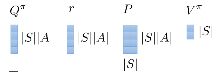
\end{split} Q π ( s , a ) Q π ( s , a ) = r ( s , a ) + γ E s ′ ∼ P ( s ′ ∣ s , a ) [ V π ( s ′ )] = r ( s , a ) + γ s ′ ∑ P ( s ′ ∣ s , a ) V π ( s ′ ) So if we write out the transition fuction P P P Q π Q^\pi Q π r r r V π V^\pi V π
Dims of each matrix Q π = r + γ P V π Q^\pi = r + \gamma PV^\pi Q π = r + γ P V π Remember that V V V Q Q Q Π ∈ R ∣ S ∣ × ( ∣ S ∣ ∣ A ∣ ) \Pi \in \mathbb{R}^{|S| \times (|S||A|)} Π ∈ R ∣ S ∣ × ( ∣ S ∣∣ A ∣ )
V π = Π Q π V^\pi = \Pi Q^\pi V π = Π Q π With this, (and P π = P Π P^\pi = P \Pi P π = P Π
Q π = r + γ P π Q π Q^\pi = r + \gamma P^\pi Q^\pi Q π = r + γ P π Q π So
( I − γ P π ) Q π = r Q π = ( I − γ P π ) − 1 r \begin{split}
(I - \gamma P^\pi)Q^\pi &= r \\
Q^\pi &= (I-\gamma P^\pi)^{-1} r
\end{split} ( I − γ P π ) Q π Q π = r = ( I − γ P π ) − 1 r And turns out the matrix ( I − γ P π ) (I - \gamma P^\pi) ( I − γ P π )
Simulation Lemma :
Q π − Q ^ π = γ ( I − γ P ^ π ) − 1 undefined Evaluation Operator: Turns reward function into Q function ( P − P ^ ) undefined Difference in model probability V π Q^\pi - \hat{Q}^\pi = \gamma \overbrace{(I-\gamma \hat{P}^\pi)^{-1}}^{\mathclap{\text{Evaluation Operator: Turns reward function into Q function}}} \underbrace{(P-\hat{P})}_{\mathclap{\text{Difference in model probability}}} V^\pi Q π − Q ^ π = γ ( I − γ P ^ π ) − 1 Evaluation Operator: Turns reward function into Q function Difference in model probability ( P − P ^ ) V π Proof:
Q π − Q ^ π = Q π − ( I − γ P ^ π ) − 1 r = ( I − γ P ^ π ) − 1 ( I − γ P ^ π ) Q π − ( I − γ P ^ π ) − 1 r = ( I − γ P ^ π ) − 1 ( I − γ P ^ π ) Q π − ( I − γ P ^ π ) − 1 ( I − γ P π ) Q π = ( I − γ P ^ π ) − 1 [ ( I − γ P ^ π ) − ( I − γ P π ) ] Q π = γ ( I − γ P ^ π ) − 1 ( P π − P ^ π ) Q π = γ ( I − γ P ^ π ) − 1 ( P Π − P ^ Π ) Q π = γ ( I − γ P ^ π ) − 1 ( P − P ^ ) Π Q π = γ ( I − γ P ^ π ) − 1 ( P − P ^ ) V π \begin{split}
Q^\pi - \hat{Q}^\pi &= Q^\pi - (I-\gamma \hat{P}^\pi)^{-1}r \\
&=(I-\gamma\hat{P}^\pi)^{-1}(I - \gamma \hat{P}^\pi)Q^\pi - (I-\gamma \hat{P}^\pi)^{-1} r \\
&=(I-\gamma\hat{P}^\pi)^{-1}(I - \gamma \hat{P}^\pi)Q^\pi - (I-\gamma \hat{P}^\pi)^{-1} (I-\gamma P^\pi) Q^\pi \\
&=(I-\gamma\hat{P}^\pi)^{-1} [(I-\gamma \hat{P}^\pi) - (I-\gamma P^\pi)] Q^\pi \\
&=\gamma(I-\gamma\hat{P}^\pi)^{-1} (P^\pi - \hat{P}^\pi)Q^\pi \\
&=\gamma(I-\gamma\hat{P}^\pi)^{-1} (P \Pi - \hat{P} \Pi)Q^\pi \\
&=\gamma(I-\gamma\hat{P}^\pi)^{-1} (P - \hat{P})\Pi Q^\pi \\
&=\gamma(I-\gamma\hat{P}^\pi)^{-1} (P- \hat{P})V^\pi \\
\end{split} Q π − Q ^ π = Q π − ( I − γ P ^ π ) − 1 r = ( I − γ P ^ π ) − 1 ( I − γ P ^ π ) Q π − ( I − γ P ^ π ) − 1 r = ( I − γ P ^ π ) − 1 ( I − γ P ^ π ) Q π − ( I − γ P ^ π ) − 1 ( I − γ P π ) Q π = ( I − γ P ^ π ) − 1 [( I − γ P ^ π ) − ( I − γ P π )] Q π = γ ( I − γ P ^ π ) − 1 ( P π − P ^ π ) Q π = γ ( I − γ P ^ π ) − 1 ( P Π − P ^ Π ) Q π = γ ( I − γ P ^ π ) − 1 ( P − P ^ ) Π Q π = γ ( I − γ P ^ π ) − 1 ( P − P ^ ) V π Another Lemma :
Given P π P^\pi P π v ⃗ ∈ R ∣ S ∣ ∣ A ∣ \vec{v} \in \mathbb{R}^{|S||A|} v ∈ R ∣ S ∣∣ A ∣
∣ ∣ ( I − γ P π ) − 1 v ⃗ ∣ ∣ ∞ ≤ ∣ ∣ v ⃗ ∣ ∣ ∞ 1 − γ ||(I-\gamma P^\pi)^{-1}\vec{v}||_\infin \le \frac{||\vec{v}||_\infin}{1-\gamma} ∣∣ ( I − γ P π ) − 1 v ∣ ∣ ∞ ≤ 1 − γ ∣∣ v ∣ ∣ ∞ “Q function” corresponding to “reward” v ⃗ \vec{v} v ( 1 − γ ) − 1 (1-\gamma)^{-1} ( 1 − γ ) − 1
Where does this ( 1 − γ ) − 1 (1-\gamma)^{-1} ( 1 − γ ) − 1 ∑ t = 0 ∞ γ t c = c 1 − γ \sum_{t=0}^\infin \gamma^t c = \frac{c}{1-\gamma} ∑ t = 0 ∞ γ t c = 1 − γ c
Let
w ⃗ = ( I γ P π ) − 1 v ⃗ \vec{w} = (I\gamma P^\pi)^{-1}\vec{v} w = ( I γ P π ) − 1 v Then
∣ ∣ v ⃗ ∣ ∣ ∞ = ∣ ∣ ( I − γ P π ) w ⃗ ∣ ∣ ∞ ≥ undefined Triangular Inequality ∣ ∣ w ⃗ ∣ ∣ ∞ − γ ∣ ∣ P π w ⃗ ∣ ∣ ∞ ≥ ∣ ∣ w ⃗ ∣ ∣ ∞ − γ ∣ ∣ w ⃗ ∣ ∣ ∞ ≥ ( 1 − γ ) ∣ ∣ w ⃗ ∣ ∣ ∞ \begin{split}
||\vec{v}||_\infin &= ||(I-\gamma P^\pi)\vec{w}||_\infin \\
&\overbrace{\ge}^{\mathclap{\text{Triangular Inequality}}} ||\vec{w}||_\infin - \gamma ||P^\pi \vec{w}||_\infin \\
&\ge ||\vec{w}||_\infin - \gamma||\vec{w}||_\infin \\
&\ge (1-\gamma) ||\vec{w}||_\infin
\end{split} ∣∣ v ∣ ∣ ∞ = ∣∣ ( I − γ P π ) w ∣ ∣ ∞ ≥ Triangular Inequality ∣∣ w ∣ ∣ ∞ − γ ∣∣ P π w ∣ ∣ ∞ ≥ ∣∣ w ∣ ∣ ∞ − γ ∣∣ w ∣ ∣ ∞ ≥ ( 1 − γ ) ∣∣ w ∣ ∣ ∞ Putting the lemmas together,
∣ ∣ ( I − γ P π ) − 1 v ⃗ ∣ ∣ ∞ ≤ ∣ ∣ v ⃗ ∣ ∣ ∞ \begin{split}
||(I-\gamma P^\pi)^{-1}\vec{v}||_\infin &\le ||\vec{v}||_\infin \\
\end{split} ∣∣ ( I − γ P π ) − 1 v ∣ ∣ ∞ ≤ ∣∣ v ∣ ∣ ∞ Let the special case v ⃗ = γ ( P − P ^ ) V π \vec{v} = \gamma(P-\hat{P})V^\pi v = γ ( P − P ^ ) V π
Q π − Q ^ π = γ ( I − γ P ^ π ) − 1 ( P − P ^ ) V π ∣ ∣ Q π − Q ^ π ∣ ∣ ∞ = ∣ ∣ γ ( I − γ P ^ π ) − 1 ( P − P ^ ) V π ∣ ∣ ∞ ≤ γ 1 − γ ∣ ∣ ( P − P ^ ) V π ∣ ∣ ∞ ≤ γ 1 − γ ( max s , a ∣ ∣ P ( ⋅ ∣ s , a ) − P ^ ( ⋅ ∣ s , a ) ∣ ∣ 1 ) ∣ ∣ V π ∣ ∣ ∞ \begin{split}
Q^\pi - \hat{Q}^\pi &= \gamma (I-\gamma \hat{P}^\pi)^{-1}(P-\hat{P})V^\pi \\
||Q^\pi - \hat{Q}^\pi||_\infin &= ||\gamma(I-\gamma \hat{P}^\pi)^{-1}(P-\hat{P})V^\pi||_\infin \\
&\le \frac{\gamma}{1-\gamma} ||(P-\hat{P})V^\pi||_\infin \\
&\le \frac{\gamma}{1-\gamma}(\max_{s,a} ||P(\cdot |s,a) - \hat{P}(\cdot|s,a)||_1) ||V^\pi||_\infin
\end{split} Q π − Q ^ π ∣∣ Q π − Q ^ π ∣ ∣ ∞ = γ ( I − γ P ^ π ) − 1 ( P − P ^ ) V π = ∣∣ γ ( I − γ P ^ π ) − 1 ( P − P ^ ) V π ∣ ∣ ∞ ≤ 1 − γ γ ∣∣ ( P − P ^ ) V π ∣ ∣ ∞ ≤ 1 − γ γ ( s , a max ∣∣ P ( ⋅ ∣ s , a ) − P ^ ( ⋅ ∣ s , a ) ∣ ∣ 1 ) ∣∣ V π ∣ ∣ ∞ We can bound ∣ ∣ V π ∣ ∣ ∞ ||V^\pi||_\infin ∣∣ V π ∣ ∣ ∞
∑ t = 0 ∞ γ t r t ≤ 1 1 − γ R m a x \sum_{t=0}^\infin \gamma^t r_t \le \frac{1}{1-\gamma}R_{max} t = 0 ∑ ∞ γ t r t ≤ 1 − γ 1 R ma x With this bound,
∣ ∣ Q π − Q ^ π ∣ ∣ ∞ ≤ γ ( 1 − γ ) 2 R m a x ( max s , a ∣ ∣ P ( ⋅ ∣ s , a ) − P ^ ( ⋅ ∣ s , a ) ∣ ∣ 1 ) ||Q^\pi-\hat{Q}^\pi||_\infin \le \frac{\gamma}{(1-\gamma)^2} R_{max} (\max_{s,a} ||P(\cdot |s,a) - \hat{P}(\cdot|s,a)||_1) ∣∣ Q π − Q ^ π ∣ ∣ ∞ ≤ ( 1 − γ ) 2 γ R ma x ( s , a max ∣∣ P ( ⋅ ∣ s , a ) − P ^ ( ⋅ ∣ s , a ) ∣ ∣ 1 ) With the previous bound on
∣ ∣ P ( ⋅ ∣ , s , a ) − P ^ ( ⋅ ∣ s , a ) ∣ ∣ 1 ≤ ∣ S ∣ N + ∣ S ∣ log ( 1 / δ ) N ≤ c ∣ S ∣ log ( 1 / δ ) N \begin{split}
||P(\cdot|,s,a) - \hat{P}(\cdot|s,a)||_1 &\le \sqrt{\frac{|S|}{N}} + \sqrt{\frac{|S|\log (1/\delta)}{N}} \\
&\le c\sqrt{\frac{|S|\log (1/\delta)}{N}}
\end{split} ∣∣ P ( ⋅ ∣ , s , a ) − P ^ ( ⋅ ∣ s , a ) ∣ ∣ 1 ≤ N ∣ S ∣ + N ∣ S ∣ log ( 1/ δ ) ≤ c N ∣ S ∣ log ( 1/ δ ) We conclude:
∣ ∣ Q π − Q ^ π ∣ ∣ ∞ ≤ ϵ = γ ( 1 − γ ) 2 R m a x c 2 ∣ S ∣ log ( δ − 1 ) N ||Q^\pi-\hat{Q}^\pi||_\infin \le \epsilon = \frac{\gamma}{(1-\gamma)^2} R_{max} c_2 \sqrt{\frac{|S| \log(\delta^{-1})}{N}} ∣∣ Q π − Q ^ π ∣ ∣ ∞ ≤ ϵ = ( 1 − γ ) 2 γ R ma x c 2 N ∣ S ∣ log ( δ − 1 ) ⚠️
Error grows
quadratically in the horizon
( 1 − γ ) − 2 (1-\gamma)^{-2} ( 1 − γ ) − 2 , each backup accumulates error
What about ∣ ∣ Q ∗ − Q ^ ∗ ∣ ∣ ∞ ||Q^* - \hat{Q}^*||_\infin ∣∣ Q ∗ − Q ^ ∗ ∣ ∣ ∞
Supremium - lower upper bound of a function (greatest value of a function), one useful identity
∣ sup x f ( x ) − sup x g ( x ) ∣ ≤ sup x ∣ f ( x ) − g ( x ) ∣ |\sup_x f(x) - \sup_x g(x)| \le \sup_x |f(x)-g(x)| ∣ x sup f ( x ) − x sup g ( x ) ∣ ≤ x sup ∣ f ( x ) − g ( x ) ∣ And
∣ ∣ Q ∗ − Q ^ ∗ ∣ ∣ ∞ = ∣ ∣ sup π Q π − sup π Q ^ π ∣ ∣ ∞ ≤ sup π ∣ ∣ Q π − Q ^ π ∣ ∣ ∞ ≤ ϵ ||Q^*-\hat{Q}^*||_\infin = ||\sup_\pi Q^\pi - \sup_\pi \hat{Q}^\pi||_\infin \le \sup_\pi ||Q^\pi - \hat{Q}^\pi||_\infin \le \epsilon ∣∣ Q ∗ − Q ^ ∗ ∣ ∣ ∞ = ∣∣ π sup Q π − π sup Q ^ π ∣ ∣ ∞ ≤ π sup ∣∣ Q π − Q ^ π ∣ ∣ ∞ ≤ ϵ What about ∣ ∣ Q ∗ − Q π ^ ∗ ∣ ∣ ∞ ||Q^* - Q^{\hat{\pi}^*}||_\infin ∣∣ Q ∗ − Q π ^ ∗ ∣ ∣ ∞
∣ ∣ Q ∗ − Q π ^ ∗ ∣ ∣ ∞ = ∣ ∣ Q ∗ − Q ^ π ^ ∗ + Q ^ π ^ ∗ − Q π ^ ∗ ∣ ∣ ∞ ≤ ∣ ∣ Q ∗ − Q ^ π ^ ∗ undefined Q ^ ∗ ∣ ∣ ∞ + ∣ ∣ Q ^ π ^ ∗ − Q π ^ ∗ undefined Same Policy ∣ ∣ ∞ ≤ 2 ϵ \begin{split}
||Q^* - Q^{\hat{\pi}^*}||_\infin &= ||Q^* - \hat{Q}^{\hat{\pi}^*}+\hat{Q}^{\hat{\pi}^*} - Q^{\hat{\pi}^*}||_\infin \\
&\le ||Q^* - \underbrace{\hat{Q}^{\hat{\pi}^*}}_{\hat{Q}^*}||_\infin + ||\underbrace{\hat{Q}^{\hat{\pi}^*} - Q^{\hat{\pi}^*}}_{\mathclap{\text{Same Policy}}}||_\infin \\
&\le 2\epsilon
\end{split} ∣∣ Q ∗ − Q π ^ ∗ ∣ ∣ ∞ = ∣∣ Q ∗ − Q ^ π ^ ∗ + Q ^ π ^ ∗ − Q π ^ ∗ ∣ ∣ ∞ ≤ ∣∣ Q ∗ − Q ^ ∗ Q ^ π ^ ∗ ∣ ∣ ∞ + ∣∣ Same Policy Q ^ π ^ ∗ − Q π ^ ∗ ∣ ∣ ∞ ≤ 2 ϵ Fixed Q-Iteration Abstract model of exact Q-iteration
Q k + 1 ← T Q k = r + γ P max a Q k Q_{k+1} \leftarrow TQ_k = r+\gamma P \max_{a} Q_k Q k + 1 ← T Q k = r + γ P a max Q k Abstract model of approximate fitted Q-iteration:
Q ^ k + 1 ← arg min Q ^ ∣ ∣ Q ^ − T ^ Q ^ k ∣ ∣ \hat{Q}_{k+1} \leftarrow \argmin_{\hat{Q}} ||\hat{Q} - \hat{T}\hat{Q}_k|| Q ^ k + 1 ← Q ^ arg min ∣∣ Q ^ − T ^ Q ^ k ∣∣ Where T ^ \hat{T} T ^
T ^ Q = r ^ undefined r ^ ( s , a ) = 1 N ( s , a ) ∑ i δ ( ( s i , a i ) = ( s , a ) ) r i + γ P ^ undefined P ^ ( s ′ ∣ s , a ) = N ( s , a , s ′ ) N ( s , a ) max a Q \hat{T}Q = \underbrace{\hat{r}}_{\mathclap{\hat{r}(s,a) = \frac{1}{N(s,a)}\sum_i \delta((s_i,a_i) = (s,a)) r_i}} + \gamma \overbrace{\hat{P}}^{\mathclap{\hat{P}(s'|s,a) = \frac{N(s,a,s')}{N(s,a)}}} \max_a Q T ^ Q = r ^ ( s , a ) = N ( s , a ) 1 ∑ i δ (( s i , a i ) = ( s , a )) r i r ^ + γ P ^ P ^ ( s ′ ∣ s , a ) = N ( s , a ) N ( s , a , s ′ ) a max Q Note: We will not be computing P ^ \hat{P} P ^ r ^ \hat{r} r ^
We will assume an infinity norm here because there will be no convergnce if using L2 norm
Erorrs come from
Q ^ k + 1 ≠ T ^ Q ^ k \hat{Q}_{k+1} \ne \hat{T}\hat{Q}_k Q ^ k + 1 = T ^ Q ^ k
Sampling Error :
∣ T ^ Q ( s , a ) − T Q ( s , a ) ∣ = ∣ r ^ ( s , a ) − r ( s , a ) + γ ( E P ^ [ max a ′ Q ( s ′ , a ′ ) ] − E P [ max a ′ Q ( s ′ , a ′ ) ] ) ∣ ≤ ∣ r ^ ( s , a ) − r ( s , a ) ∣ + γ ∣ E P ^ [ max a ′ Q ( s ′ , a ′ ) ] − E P [ max a ′ Q ( s ′ , a ′ ) ] ∣ \begin{split}
|\hat{T}Q(s,a) - TQ(s,a)| &= |\hat{r}(s,a)-r(s,a)+\gamma(\mathbb{E}_{\hat{P}}[\max_{a'} Q(s',a')] - \mathbb{E}_{P}[\max_{a'} Q(s',a')])| \\
&\le |\hat{r}(s,a) - r(s,a)| + \gamma {|\mathbb{E}_{\hat{P}}[\max_{a'}Q(s',a')]-\mathbb{E}_{P}[\max_{a'}Q(s',a')]|} \\
\end{split} ∣ T ^ Q ( s , a ) − TQ ( s , a ) ∣ = ∣ r ^ ( s , a ) − r ( s , a ) + γ ( E P ^ [ a ′ max Q ( s ′ , a ′ )] − E P [ a ′ max Q ( s ′ , a ′ )]) ∣ ≤ ∣ r ^ ( s , a ) − r ( s , a ) ∣ + γ ∣ E P ^ [ a ′ max Q ( s ′ , a ′ )] − E P [ a ′ max Q ( s ′ , a ′ )] ∣ Note:
∣ r ^ ( s , a ) − r ( s , a ) ∣ |\hat{r}(s,a) - r(s,a)| ∣ r ^ ( s , a ) − r ( s , a ) ∣ Estimation error of continuous random variable, use Hoeffding’s Inequality! ≤ 2 R m a x log ( δ − 1 ) 2 N \le 2 R_{max} \sqrt{\frac{\log (\delta^{-1})}{2N}} ≤ 2 R ma x 2 N l o g ( δ − 1 ) ∣ E P ^ [ max a ′ Q ( s ′ , a ′ ) ] − E P [ max a ′ Q ( s ′ , a ′ ) ] ∣ |\mathbb{E}{\hat{P}}[\max{a'}Q(s',a')]-\mathbb{E}{P}[\max{a'}Q(s',a')]| ∣ E P ^ [ max a ′ Q ( s ′ , a ′ )] − E P [ max a ′ Q ( s ′ , a ′ )] ∣ = ∑ s ’ ( P ^ ( s ’ ∣ s , a ) − P ( s ’ ∣ s , a ) ) max a ’ Q ( s ’ , a ’ ) = \sum_{s’} (\hat{P}(s’|s,a) - P(s’|s,a)) \max_{a’} Q(s’,a’) = ∑ s ’ ( P ^ ( s ’∣ s , a ) − P ( s ’∣ s , a )) max a ’ Q ( s ’ , a ’ ) ≤ ∑ s ’ ∣ P ^ ( s ’ ∣ s , a ) − P ( s ’ ∣ s , a ) ∣ max s ’ , a ’ Q ( s ’ , a ’ ) \le \sum_{s’} |\hat{P}(s’|s,a) - P(s’|s,a)| \max_{s’,a’} Q(s’,a’) ≤ ∑ s ’ ∣ P ^ ( s ’∣ s , a ) − P ( s ’∣ s , a ) ∣ max s ’ , a ’ Q ( s ’ , a ’ ) = ∣ ∣ P ^ ( ⋅ ∣ s , a ) − P ( ⋅ ∣ s , a ) ∣ ∣ 1 ∣ ∣ Q ∣ ∣ ∞ = ||\hat{P}(\cdot|s,a) - P(\cdot|s,a)||_1 ||Q||_\infin = ∣∣ P ^ ( ⋅ ∣ s , a ) − P ( ⋅ ∣ s , a ) ∣ ∣ 1 ∣∣ Q ∣ ∣ ∞ ≤ c ∣ ∣ Q ∣ ∣ ∞ log ( δ − 1 ) N \le c||Q||_\infin \sqrt{\frac{\log(\delta^{-1})}{N}} ≤ c ∣∣ Q ∣ ∣ ∞ N l o g ( δ − 1 ) So
∣ T ^ Q ( s , a ) − T Q ( s , a ) ∣ ≤ 2 R m a x log ( δ − 1 ) 2 N + c ∣ ∣ Q ∣ ∣ ∞ log ( δ − 1 ) N |\hat{T}Q(s,a) -TQ(s,a)| \le 2R_{max} \sqrt{\frac{\log(\delta^{-1})}{2N}} + c||Q||_\infin \sqrt{\frac{\log(\delta^{-1})}{N}} ∣ T ^ Q ( s , a ) − TQ ( s , a ) ∣ ≤ 2 R ma x 2 N log ( δ − 1 ) + c ∣∣ Q ∣ ∣ ∞ N log ( δ − 1 ) And
∣ ∣ T ^ Q − T Q ∣ ∣ ∞ ≤ 2 R m a x c 1 log ( ∣ S ∣ ∣ A ∣ δ ) 2 N + c 2 ∣ ∣ Q ∣ ∣ ∞ log ( ∣ S ∣ δ ) N ||\hat{T}Q - TQ||_\infin \le 2R_{max} c_1 \sqrt{\frac{\log(\frac{|S||A|}{\delta})}{2N}} + c_2||Q||_\infin \sqrt{\frac{\log(\frac{|S|}{\delta})}{N}} ∣∣ T ^ Q − TQ ∣ ∣ ∞ ≤ 2 R ma x c 1 2 N log ( δ ∣ S ∣∣ A ∣ ) + c 2 ∣∣ Q ∣ ∣ ∞ N log ( δ ∣ S ∣ )
Approximation Error :
Assume error: ∣ ∣ Q ^ k + 1 − T Q ^ k ∣ ∣ ∞ ∣ ∣ ∞ ≤ ϵ k ||\hat{Q}_{k+1} - T\hat{Q}_k||_\infin||_\infin \le \epsilon_k ∣∣ Q ^ k + 1 − T Q ^ k ∣ ∣ ∞ ∣ ∣ ∞ ≤ ϵ k
This is a strong assumption!
∣ ∣ Q ^ k − Q ∗ ∣ ∣ ∞ = ∣ ∣ Q ^ k − T Q ^ k − 1 + T Q ^ k − 1 − Q ∗ ∣ ∣ ∞ = ∣ ∣ ( Q ^ k − T Q ^ k − 1 ) + ( T Q ^ k − 1 − T Q ∗ undefined Using the fact that Q ∗ is a fixed point of T ) ∣ ∣ ∞ ≤ ∣ ∣ Q ^ k − T Q ^ k − 1 ∣ ∣ ∞ + ∣ ∣ T Q ^ k − 1 − T Q ∗ ∣ ∣ ∞ ≤ ϵ k − 1 + γ ∣ ∣ Q ^ k − 1 − Q ∗ ∣ ∣ ∞ undefined Using the fact that T is a γ -contraction Unroll the recursion, ≤ ∑ i = 0 k − 1 γ i ϵ k − i − 1 + γ ∣ ∣ Q ^ k − 1 − Q ∗ ∣ ∣ ∞ \begin{split}
||\hat{Q}_k - Q^*||_\infin
&= ||\hat{Q}_k - T\hat{Q}_{k-1} + T\hat{Q}_{k-1}-Q^*||_\infin \\
&= ||(\hat{Q}_k - T\hat{Q}_{k-1}) + (T\hat{Q}_{k-1} - \underbrace{TQ^*}_{\mathclap{\text{Using the fact that $Q^*$ is a fixed point of $T$}}})||_\infin \\
&\le ||\hat{Q}_k - T\hat{Q}_{k-1}||_\infin + ||T\hat{Q}_{k-1} - TQ^*||_\infin \\
&\le \epsilon _{k-1} + \underbrace{\gamma ||\hat{Q}_{k-1}- Q^*||_\infin}_{\mathclap{\text{Using the fact that $T$ is a $\gamma$-contraction}}} \\
\text{Unroll the recursion,} \\
&\le \sum_{i=0}^{k-1} \gamma^i \epsilon_{k-i-1} + \gamma ||\hat{Q}_{k-1} - Q^*||_\infin \\
\end{split} ∣∣ Q ^ k − Q ∗ ∣ ∣ ∞ Unroll the recursion, = ∣∣ Q ^ k − T Q ^ k − 1 + T Q ^ k − 1 − Q ∗ ∣ ∣ ∞ = ∣∣ ( Q ^ k − T Q ^ k − 1 ) + ( T Q ^ k − 1 − Using the fact that Q ∗ is a fixed point of T T Q ∗ ) ∣ ∣ ∞ ≤ ∣∣ Q ^ k − T Q ^ k − 1 ∣ ∣ ∞ + ∣∣ T Q ^ k − 1 − T Q ∗ ∣ ∣ ∞ ≤ ϵ k − 1 + Using the fact that T is a γ -contraction γ ∣∣ Q ^ k − 1 − Q ∗ ∣ ∣ ∞ ≤ i = 0 ∑ k − 1 γ i ϵ k − i − 1 + γ ∣∣ Q ^ k − 1 − Q ∗ ∣ ∣ ∞
lim k → ∞ ∣ ∣ Q ^ k − Q ∗ ∣ ∣ ∞ ≤ ∑ i = 0 ∞ γ i max k ϵ k = 1 1 − γ ∣ ∣ ϵ ∣ ∣ ∞ \lim_{k \to \infin} ||\hat{Q}_k - Q^*||_\infin \le \sum_{i=0}^{\infin} \gamma^i \max_{k} \epsilon_k = \frac{1}{1-\gamma}||\epsilon||_\infin k → ∞ lim ∣∣ Q ^ k − Q ∗ ∣ ∣ ∞ ≤ i = 0 ∑ ∞ γ i k max ϵ k = 1 − γ 1 ∣∣ ϵ ∣ ∣ ∞
Putting it together:
∣ ∣ Q ^ k − T Q ^ k − 1 ∣ ∣ ∞ = ∣ ∣ Q ^ k − T ^ Q ^ k − 1 + T ^ Q ^ k − 1 − T Q ^ k − 1 ∣ ∣ ∞ ≤ ∣ ∣ Q ^ k − T ^ Q ^ k − 1 ∣ ∣ ∞ undefined Approximation Error + ∣ ∣ T ^ Q ^ k − 1 − T Q ^ k − 1 ∣ ∣ ∞ undefined Sampling Error \begin{split}
||\hat{Q}_k - T\hat{Q}_{k-1}||_\infin
&= ||\hat{Q}_k - \hat{T}\hat{Q}_{k-1} + \hat{T}\hat{Q}_{k-1} - T\hat{Q}_{k-1}||_\infin \\
&\le \underbrace{||\hat{Q}_k - \hat{T}\hat{Q}_{k-1}||_\infin}_{\mathclap{\text{Approximation Error}}} + \underbrace{||\hat{T}\hat{Q}_{k-1} - T\hat{Q}_{k-1}||_\infin}_{\mathclap{\text{Sampling Error}}} \\
\end{split} ∣∣ Q ^ k − T Q ^ k − 1 ∣ ∣ ∞ = ∣∣ Q ^ k − T ^ Q ^ k − 1 + T ^ Q ^ k − 1 − T Q ^ k − 1 ∣ ∣ ∞ ≤ Approximation Error ∣∣ Q ^ k − T ^ Q ^ k − 1 ∣ ∣ ∞ + Sampling Error ∣∣ T ^ Q ^ k − 1 − T Q ^ k − 1 ∣ ∣ ∞ Note:
From previous proofs, Sampling Error , Approx Error ∈ O ( ( 1 − γ ) − 1 ) \text{Sampling Error}, \text{Approx Error} \in O((1-\gamma)^{-1}) Sampling Error , Approx Error ∈ O (( 1 − γ ) − 1 )
More advanced results can be derived with p p p